ポータルサイト

GenomeMatcher version 3 について

macOS10.15にて32 bitのプログラムが動作しなくなりました(GenomeMatcherでは内包するbl2seq等を利用していましたが、これらが動作しなくなりました)。このためGenomeMatcherをアップデートし、version 3.0としました。

使用するblastプログラムはいずれもblast+の2.9.0+になりました。また、MUMmer、MADDT、CONSERV、clustalW2はユーザー自身でダウンロードし、プログラムへのパスを指定する必要があります。
メイン画面をリサイズ可能にしました。ディスプレイを広く使って解析することができます。
メイン画面で遺伝子の表示トラックを2つに増やしました。
認証システムを変更しました。MACアドレスが変更されるのに伴って起動キーを取得し直さなくてはならない問題が解決されています。
様々な変更を加えましたので、不具合が残っている可能性があります。問題をご報告いただけますと助かります。
エクセルからデータをコピーペーストで入力した際の不具合を解消しました(version3.05)

起動した時に、「アプリケーションは壊れているために開けません」とのエラーが出ることがあります。この場合ターミナルを開き、

xattr -rc /Users/user_name/Downloads/GenomeMatcher3.07.app

などとしてください。xattr -rc と打ち込んだ後に、アプリケーションのアイコンをドラッグすると簡単です。-rcの前後に半角スペースが必要ですので注意してください。

作者: 東北大学大学院生命科学研究科准教授　大坪嘉行

GenomeMatcher 3.10 Download <update 2024.08.28 (OS10.10以降のみ)>

メイン画面で、比較解析結果が表示されないエラーを修正しました(サムネイル画像をクリックして、比較対象配列を変更した場合に起きるエラーでした)。

更新情報等は、ツイッターからも配信予定です。

アカウント: @GenomeMatcher

旧ページへのリンク

本書では、科学的素養を7項目で整理・明文化しています。教育の質、学びの質を高め、研究力向上を。
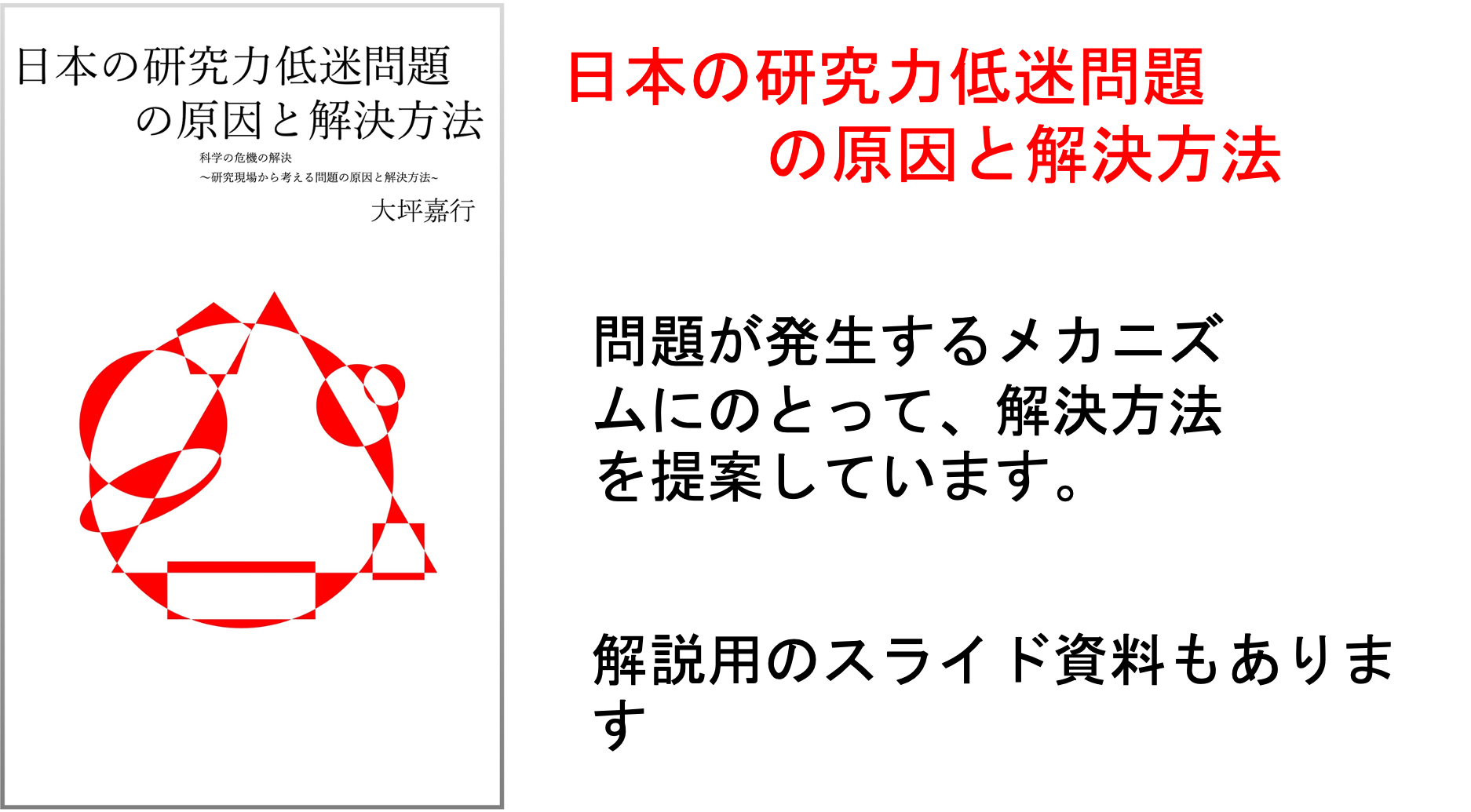本書では、研究力低迷問題を分析し、解決策を提案しています。研究、教育に携わる多くの方にお読みいただけますと幸いです。解説資料平易版・提案資料
QRコードをスマホで読み取って出席登録。出席管理WEBシステムです。
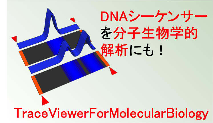TraceViewer。変性ポリアクリルアミドゲル電気泳動の代わりにシーケンサーでデータを取りませんか？macOSアプリです。
ShortReadManager NGSデータの処理に便利なmacOSアプリです。変なアイコンですみません。
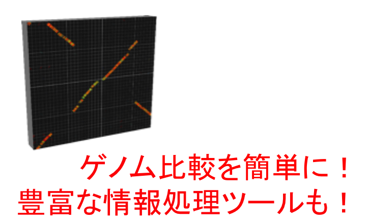GenomeMatcher ゲノム比較機能をはじめ色々な情報処理ツールがついています。数値データをグラフィックスに変換する機能も。
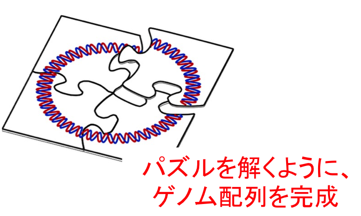GenoFinisher バクテリアゲノムをshort readだけでも決定可能です。バクテリアゲノムのフィニッシングでお困りの方はご相談ください。
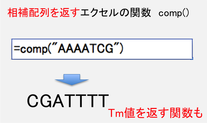DNA配列の相補配列を計算する関数を含むエクセルシートです。
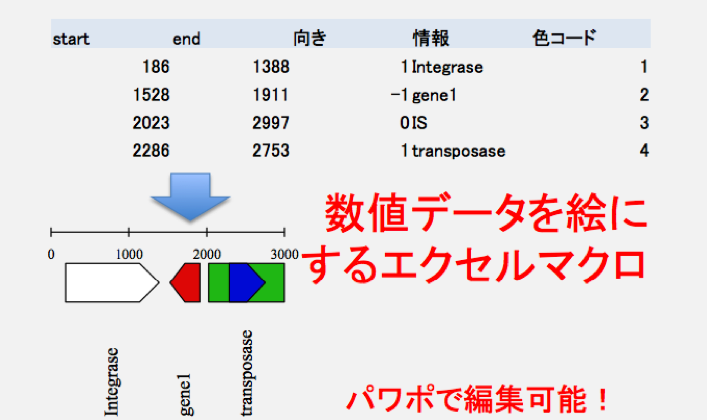数値データを絵に変換するマクロを含むエクセルシートです。
数値データを元にサーキュラーマップが描けます。データ生成機能もあります。
大学等研究機関での実験機器類の共用を促進するためのウエブシステムです。
DNA配列/アミノ酸配列を2次元パネルの上で動かせるソフトウエアです。配列比較も。
例の処理を簡単に済ませるあのツールです。
iPhoneアプリです。勤務地への入域と出域時刻のログを自動的にとります。App Storeから入手できます。
文字列集合を取り扱える便利ツールです。
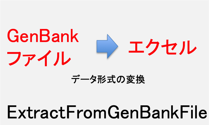GenBankファイルのデータを、エクセルシートで取り扱えるように変換するツールです。
文字列を取り扱える便利ツールです。
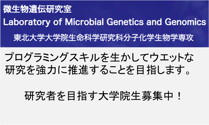作者研究室ホームページ。共同研究の提案と研究室への寄付を歓迎します。

作者プロフィール: 環境細菌の研究を進める一方で、様々なソフトウエアを作成、公開している。